House price prediction is a problem in the real estate industry to make informed decisions. By using machine learning algorithms we can predict the price of a house based on various features such as location, size, number of bedrooms and other relevant factors. In this article we will explore how to build a machine learning model in Python to predict house prices to gain valuable insights into the housing market.
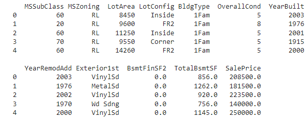
To tackle this issue we will build a machine learning model trained on the House Price Prediction Dataset. We can download the dataset from the provided link. It includes 13 features:
| Id | To count the records. |
|---|---|
| MSSubClass | Identifies the type of dwelling involved in the sale. |
| MSZoning | Identifies the general zoning classification of the sale. |
| LotArea | Lot size in square feet. |
| LotConfig | Configuration of the lot |
| BldgType | Type of dwelling |
| OverallCond | Rates the overall condition of the house |
| YearBuilt | Original construction year |
| YearRemodAdd | Remodel date (same as construction date if no remodeling or additions). |
| Exterior1st | Exterior covering on house |
| BsmtFinSF2 | Type 2 finished square feet. |
| TotalBsmtSF | Total square feet of basement area |
| SalePrice | To be predicted |
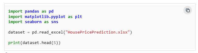
Step 1: Importing Libraries and Dataset
In the first step we load the libraries which is needed for Prediction:
- Pandas – To load the Dataframe
- Matplotlib – To visualize the data features i.e. barplot
- Seaborn – To see the correlation between features using heatmap
As we have imported the data. So shape method will show us the dimension of the dataset.
dataset.shape
(2919,13)
Step 2: Data Preprocessing
Now, we categorize the features depending on their datatype (int, float, object) and then calculate the number of them.
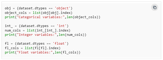
Output:
Categorical variables : 4
Integer variables : 6
Float variables : 3
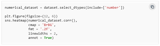
Step 3: Exploratory Data Analysis
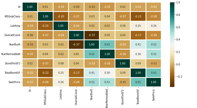
EDA refers to the deep analysis of data so as to discover different patterns and spot anomalies. Before making inferences from data it is essential to examine all your variables. So here let’s make a heatmap using seaborn library.
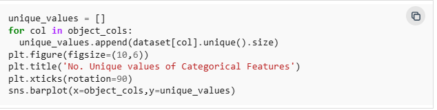
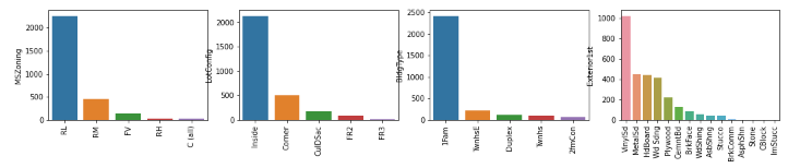
To analyze the different categorical features. Let’s draw the barplot.
Output:
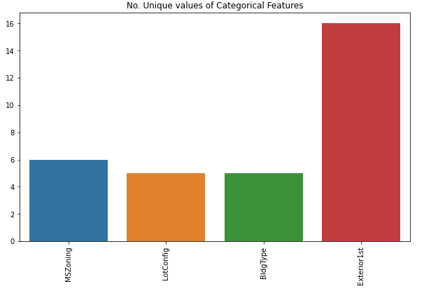
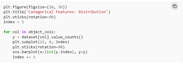
The plot shows that Exterior1st has around 16 unique categories and other features have around 6 unique categories. To findout the actual count of each category we can plot the bargraph of each four features separately.
Output:
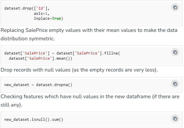
Step 4: Data Cleaning
Data Cleaning is the way to improvise the data or remove incorrect, corrupted or irrelevant data. As in our dataset there are some columns that are not important and irrelevant for the model training. So we can drop that column before training. There are 2 approaches to dealing with empty/null values
- We can easily delete the column/row (if the feature or record is not much important).
- Filling the empty slots with mean/mode/0/NA/etc. (depending on the dataset requirement).
As Id Column will not be participating in any prediction. So we can Drop it.
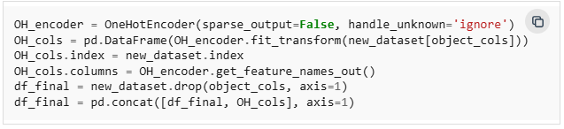
Step 5: OneHotEncoder – For Label categorical features
One hot Encoding is the best way to convert categorical data into binary vectors. This maps the values to integer values. By using OneHotEncoder, we can easily convert object data into int. So for that firstly we have to collect all the features which have the object datatype. To do so, we will make a loop.
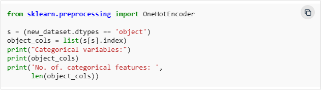
Output:

Then once we have a list of all the features. We can apply OneHotEncoding to the whole list.
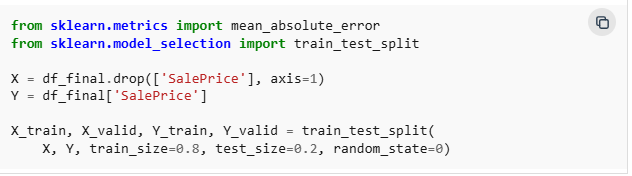
Step 6: Splitting Dataset into Training and Testing
X and Y splitting (i.e. Y is the SalePrice column and the rest of the other columns are X)
Step 7: Model Training and Accuracy
As we have to train the model to determine the continuous values, so we will be using these regression models.
- SVM-Support Vector Machine
- Random Forest Regressor
- Linear Regressor
And To calculate loss we will be using the mean_absolute_percentage_error module. It can easily be imported by using sklearn library. The formula for Mean Absolute Error is:
![]()
1. SVM – Support vector Machine
Support vector Machine is a supervised machine learning algorithm primarily used for classification tasks though it can also be used for regression. It works by finding the hyperplane that best divides a dataset into classes. The goal is to maximize the margin between the data points and the hyperplane.
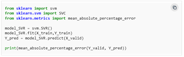
Output :
0.18705129
2. Random Forest Regression
Random Forest is an ensemble learning algorithm used for both classification and regression tasks. It constructs multiple decision trees during training where each tree in the forest is built on a random subset of the data and features, ensuring diversity in the model. The final output is determined by averaging the outputs of individual trees (for regression) or by majority voting (for classification).
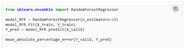
Output :
0.1929469
3. Linear Regression
Linear Regression is a statistical method used for modeling the relationship between a dependent variable and one or more independent variables. The goal is to find the line that best fits the data. This is done by minimizing the sum of the squared differences between the observed and predicted values. Linear regression assumes that the relationship between variables is linear.
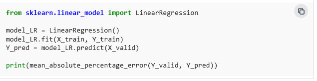
Output :
0.187416838
Clearly SVM model is giving better accuracy as the mean absolute error is the least among all the other regressor models i.e. 0.18 approx. To get much better results ensemble learning techniques like Bagging and Boosting can also be used.