How Computers “See” Molecules

To a computer, Edvard Munch’s The Scream is nothing more than a grid of pixel values. It has no sense of why swirling lines in a twilight sky convey the agony of a scream. That’s because (modern digital) computers fundamentally process only binary signals [1,2]; they don’t inherently comprehend the objects and emotions we perceive.

To mimic human intelligence, we first need an intermediate form (representation) to “translate” our sensory world into something a computer can handle. For The Scream, that might mean extracting edges, colors, shapes, etc. Likewise, in Natural Language Processing (NLP), a computer sees human language as an unstructured stream of symbols that must be turned into numeric vectors or other structured forms. Only then can it begin to map raw input to higher-level concepts (i.e., building a model).

Human intelligence also depends on internal representations.

In psychology, a representation refers to an internal mental symbol or image that stands for something in the outside world [3]. In other words, a representation is how information is encoded in the brain: the symbols we use (words, images, memories, artistic depictions, etc.) to stand for objects and ideas.

Our senses don’t simply put the external world directly into our brains; instead, they convert sensory input into abstract neural signals. For example, the eyes convert light into electrical signals on the retina, and the ears turn air vibrations into nerve impulses. These neural signals are the brain’s representation of the external world, which is used to reconstruct our perception of reality, essentially building a “model” in our mind.

Between ages one and two, children enter Piaget’s early preoperational stage [4]. This is when kids start using one thing to represent another: a toddler might hold a banana up to their ear and babble as if it’s a phone, or push a box around pretending it’s a car. This kind of symbolic play is important for cognitive development, because it shows the child can move beyond the here-and-now and project the concepts in their mind onto reality [5].

Without our senses translating physical signals into internal codes, we couldn’t perceive anything [5].

“Garbage in, garbage out”. The quality of a representation sets an upper bound on the performance of any model built on it [6,7].

Much of the progress in human intelligence has come from improving how we represent knowledge [8].

One of the core goals of education is to help students form effective mental representations of new knowledge. Seasoned educators use diagrams, animations, analogies and other tools to present abstract concepts in a vivid, relatable way. Richard Mayer argues that meaningful learning happens when learners form a coherent mental representation or model of the material, rather than just memorizing disconnected facts [8]. In meaningful learning, new information integrates into existing knowledge, allowing students to transfer and apply it in novel situations.

However, in practice, factors like limited model capacity and finite computing resources constrain how complex our representations can be. Compressing input data inevitably risks information loss, noise, and artifacts. So, as the first step, developing a “good enough” representation requires balancing several key properties:

• It should retain the information critical to the task. (A clear problem definition helps filter out the rest.)
• It should be as compact as possible: minimizing redundancy and keeping dimensionality low.
• It should separate classes in feature space. Samples from the same class cluster together, while those from different classes stay far apart.
• It should be robust to input noise, compression artifacts, and shifts in data modality.
• Invariance. Representations should be invariant to task‑irrelevant changes (e.g. rotating or translating an image, or changing its brightness).
• Generalizability.
• Interpretability.
• Transferability.

These limitations on representation complexity are somewhat analogous to the limited capacity of our own working memory.

Human short-term memory, on average, can only hold about 7±2 items at once [9]. When too many independent pieces of information arrive simultaneously (beyond what our cognitive load can handle), our brains bog down. Cognitive psychology research shows that with the right guidance (by adjusting how information is represented), people can reorganize information to overcome this apparent limit [10,11]. For example, we can remember a long string of digits more easily by chunking them into meaningful groups (which is why phone numbers are often split into shorter blocks).

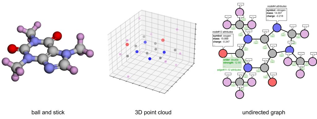
Now, shifting from The Scream to the microscopic world of molecules, we face the same challenge: how can we translate real-world molecules into a form that a computer can understand? With the right representation, a computer can infer chemical properties or biological functions, and ultimately map those to higher‑level concepts (e.g., a drug’s activity or a molecule’s protein binding). In this article, we’ll explore the common methods that let computers “see” molecules.

Chemical Formula

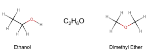
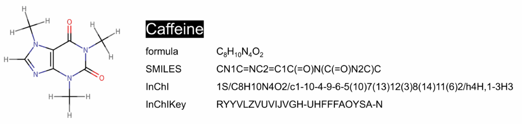
Perhaps the most straightforward depiction of a molecule is its chemical formula, like C₈H₁₀N₄O₂ (caffeine), which tells us there are 8 carbon atoms, 10 hydrogen atoms, 4 nitrogen atoms and 2 oxygen atoms. However, its very simplicity is also its limitation: a formula conveys nothing about how those atoms are connected (the bonding topology), how they are arranged in space, or where functional groups are located. That’s why isomers (like ethanol and dimethyl ether) both share C₂H₆O yet differ completely in structure and properties.

Linear String

Another common way to represent molecules is to encode them as a linear string of characters, a format widely adopted in databases [12,13].

SMILES

The most classic example is SMILES (Simplified Molecular Input Line Entry System) [14], developed by David Weininger in the 1980s. SMILES treats atoms as nodes and bonds as edges, then “flattens” them into a 1D string via a depth‑first traversal, preserving all the connectivity and ring information. Single, double, triple, and aromatic bonds are denoted by the symbols “-”, “=”, “#”, and “:”, respectively. Numbers are used to mark the start and end of rings, and branches off the main chain are enclosed in parentheses. (See more in SMILES – Wikipedia.)

SMILES is simple, intuitive, and compact for storage. Its extended syntax supports stereochemistry and isotopes. There is also a rich ecosystem of tools supporting it: most chemistry libraries let us convert between SMILES and other standard formats.

However, without an agreed-upon canonicalization algorithm, the same molecule can be written in multiple valid SMILES forms. This can potentially lead to inconsistencies or “data pollution”, especially when merging data from multiple sources.

InChI

Another widely used string format is InChI (International Chemical Identifier) [15], introduced by IUPAC in 2005, to generate globally standardized, machine-readable, and unique molecule identifiers. InChI strings, though longer than SMILES, encode more details in layers (including atoms and their bond connectivity, tautomeric state, isotopes, stereochemistry, and charge), each with strict rules and priority. (See more in InChI – Wikipedia.)

Because an InChI string can become very lengthy as a molecule grows more complex, it is often paired with a 27‑character InChIKey hash [15]. The InChIKeys aren’t human‑friendly, but they’re ideal for database indexing and for exchanging molecule identifiers across systems.

Molecular Descriptor

Many computational models require numeric inputs. Compared to linear string representations, molecular descriptors turn a molecule’s properties and patterns into a vector of numerical features, delivering satisfactory performance in many tasks [7, 16-18].

Todeschini and Consonni describe the molecular descriptor as the “final result of a logical and mathematical procedure, which transforms chemical information encoded within a symbolic representation of a molecule into a useful number or the result of some standardized experiment” [16].

We can think of a set of molecular descriptors as a standardized “physical exam sheet” for a molecule, asking questions like:

• Does it have a benzene ring?
• How many carbon atoms does it have?
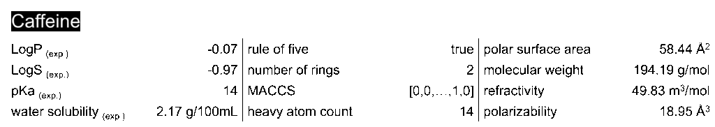
• What’s the predicted octanol-water partition coefficient (LogP)?
• Which functional groups are present?
• What is its 3D conformation or electron distribution like?
• …

Their answers can take various forms, such as numerical values, categorical flags, vectors, graph-based structures, tensors etc. Because every molecule in our dataset is described using the same set of questions (the same “physical exam sheet”), comparisons and model inputs become straightforward. And because each feature has a clear meaning, descriptors improve the interpretability of the model.

Of course, just as a physical exam sheet can’t capture absolutely everything about a person’s health, a finite set of molecular descriptors can never capture all aspects of a molecule’s chemical and physical nature. Computing descriptors is typically a non-invertible process, inevitably leading to a loss of information, and the results are not guaranteed to be unique. Therefore, there are different types of molecular descriptors, each focusing on different aspects.

Thousands of molecular descriptors have been developed over the years (for example, RDKit [19], CDK [20], Mordred [17], etc.). They can be broadly categorized by the dimensionality of information they encode (these categories aren’t strict divisions):

• 0D: formula‑based properties independent of structure (e.g., atom counts or molecular weight).
• 1D: sequence-based properties (e.g., counts of certain functional groups).
• 2D: derived from the 2D topology (e.g., eccentric connectivity index [21]).
• 3D: derived from 3D conformation, capturing geometric or spatial properties (e.g., charged partial surface area [22]).
• 4D and higher: these incorporate additional dimensions such as time, ensemble, or environmental factors (e.g., descriptors derived from molecular dynamics simulations, or from quantum chemical calculations like HOMO/LUMO).
• Descriptors obtained from other sources including experimental measurements.

Molecular fingerprints are a special kind of molecular descriptor that encode substructures into a fixed-length numerical vector [16]. This table summarizes some commonly used molecular fingerprints [23], such as MACCS [24], which is shown in the figure below.

Similarly, human fingerprints or product barcodes can also be seen as (or converted to) fixed-format numerical representations.

Different descriptors describe molecules from various aspects, so their contributions to different tasks naturally vary. In a task of predicting the aqueous solubility of drug-like molecules, over 4,000 computed descriptors were evaluated, but only about 800 made significant contributions to the prediction [7].

Point Cloud

Sometimes, we need our models to learn directly from a molecule’s 3D structure. For example, this is important when we’re interested in how two molecules might interact with each other [25], need to search the possible conformations of a molecule [26], or want to simulate its behavior in a certain environment [27].

One straightforward way to represent a 3D structure is as a point cloud of its atoms [28]. In other words, a point cloud is a collection of coordinates of the atoms in 3D space. However, while this representation shows which atoms are near each other, it doesn’t explicitly tell us which pairs of atoms are bonded. Inferring connectivity from interatomic distances (e.g., via cutoffs) can be error-prone, and may miss higher‑order chemistry like aromaticity or conjugation. Moreover, our model must account for changes of raw coordinates due to rotation or translation. (More on this later.)

Graph

A molecule can also be represented as a graph, where atoms (nodes) are connected by bonds (edges). Graph representations elegantly handle rings, branches, and complex bonding arrangements. For example, in a SMILES string, a benzene ring must be “opened” and denoted by special symbols, whereas in a graph, it’s simply a cycle of nodes connected in a loop.

Molecules are commonly modeled as undirected graphs (since bonds have no inherent direction) [29-31]. We can further “decorate” the graph with additional domain-specific knowledge to make the representation more interpretable: tagging nodes with atom features (e.g., element type, charge, aromaticity) and edges with bond properties (e.g., order, length, strength). Therefore,

• (uniqueness) each distinct molecular structure could correspond to a unique graph, and
• (reversibility) we could reconstruct the original molecule from its graph representation

Chemical reactions essentially involve breaking bonds and forming new ones. Using graphs makes it easier to track these changes. Some reaction‑prediction models encode reactants and products as graphs and infer the transformation by comparing them [32,33].

Graph Neural Networks (GNNs) can directly process graphs and learn from them. Using molecular graph representation, these models can naturally handle molecules of arbitrary size and topology. In fact, many GNNs have outperformed models that only relied on descriptors or linear strings on many molecular tasks [7,30,34].

Often, when a GNN makes a prediction, we can inspect which parts of the graph were most influential. These “important bits” frequently correspond to actual chemical substructures or functional groups. In contrast, if we were looking at a particular substring of a SMILES, it’s not guaranteed to map neatly to a meaningful substructure.

A graph doesn’t always mean just the direct bonds connecting atoms. We can construct different kinds of graphs from molecular data depending on our needs, and sometimes these alternate graphs yield better results for particular applications. For example:

Complete graph: Every pair of nodes is connected by an edge. It could introduce redundant connections, but might be used to let a model consider all pairwise interactions.
Bipartite graph: Nodes are divided into two sets, and edges only connect nodes from one set to nodes from the other.
Nearest-neighbor graph: Each node is connected only to its nearest neighbors (according to some criterion), for controlling complexity.

Extensible Graph Representations

We can incorporate chemical rules or impose constraints within molecular graphs. In de novo molecular design, (early) SMILES‑based generative models often produced SMILES strings ended up proposing invalid molecules, because: (1) assembling characters may break SMILES syntax, and (2) even a syntactically correct SMILES might encode an impossible structure. Graph‑based generative models avoid them by building molecules atom by atom and bond by bond (under user-specified chemical rules). Graphs also let us impose constraints: require or forbid specific substructures, enforce 3D shapes or chirality, and so on; thus, to guide generation toward valid candidates that meet our goals [35,36].

Molecular graphs can also handle multiple molecules and their interactions (e.g., drug-protein binding, protein-protein interfaces). “Graph-of-graphs” treat each molecule as its own graph, then deploy a higher-level model to learn how they interact [37]. Or, we may merge the molecules into one composite graph, including all atoms from both partners and add special (dummy) edges or nodes to mark their contacts [38].

So far, we’ve been considering the standard graph of bonds (the 2D connectivity), but what if the 3D arrangement matters? Graph representations can certainly be augmented with 3D information: 3D coordinates could be attached to each node, or distances/angles could be added as attributes on the edges, to make models more sensitive to difference in 3D configurations. A better option is to use models like SE(3)-equivariant GNNs, which ensure their outputs (or key internal features) transform (or stay invariant) with any rotation or translation of the input.

In 3D space, the special Euclidean group SE(3) describes all possible rigid motions (any combination of rotations and translations). (It’s sometimes described as a semidirect product of the rotation group SO(3) with the translation group R³.) [28]

When we say a model or a function has SE(3) invariance, we mean that it gives the same result no matter how we rotate or translate the input in 3D. This kind of invariance is often an essential requirement for many molecular modeling tasks: a molecule floating in solution has no fixed reference frame (i.e., it can tumble around in space). So, if we predict some property of the molecule (say its binding affinity), that prediction should not be influenced by the molecule’s orientation or position.

Sequence Representations of Biomacromolecules

We’ve talked mostly about small molecules. But biological macromolecules (like proteins, DNA, and RNA) can contain thousands or even millions of atoms. SMILES or InChI strings become extremely long and complex, leading to the associated massive computational, storage, and analysis costs.

This brings us back to the importance of defining the problem: for biomacromolecules, we’re often not interested in the precise position of every single atom or the exact bonds between each pair of atoms. Instead, we care about higher-level structural patterns and functional modules: like a protein’s amino acid backbone and its alpha‑helices or beta‑sheets, which fold into tertiary and quaternary structures. For DNA and RNA, we may care about nucleotide sequences and motifs.

We describe these biological polymers as sequences of their building blocks (i.e., primary structure): proteins as chains of amino acids, and DNA/RNA as strings of nucleotides. There are well-established codes for these building blocks (defined by IUPAC/IUBMB): for instance, in DNA, the letters A, C, G, T represent the bases adenine, cytosine, guanine, and thymine respectively.

Static Embeddings and Pretrained Embeddings

To convert a sequence into numerical vectors, we can use static embeddings: assigning a fixed vector to each residue (or k-mer fragment). The simplest static embedding is one-hot encoding (e.g., encode adenine A as [1,0,0,0]), turning a sequence into a matrix. Another approach is to learn dense (pretrained) embeddings by leveraging large databases of sequences. For example, ProtVec [39] breaks proteins into overlapping 3‑mers and trains a Word2Vec‑like model (commonly used in NLP) on a large corpus of sequences, assigning each 3-mer a 100D vector. These learned fragment embeddings are shown to capture biochemical and biophysical patterns: fragments with similar functions or properties cluster closer in the embedding space.

k-mer fragments (or k-mers) are substrings of length k extracted from a biological sequence.

Tokens

Inspired by NLP, we can treat a sequence as if it’s a sentence composed of tokens or words (i.e., residues or k-mer fragments), and then feed them into deep language models. Trained on massive collections of sequences, these models learn biology’s “grammar” and “semantics” just as they do in human language.

Transformers can use self‑attention to capture long‑range dependencies in sequences; and we essentially use them to learn a “language of biology”. (Some) Meta’s ESM series of models [40-42] trained Transformers on hundreds of millions of protein sequences. Similarly, DNABERT [43] tokenizes DNA into k‑mers for BERT training on genomic data. These kinds of obtained embeddings have been shown to encapsulate a wealth of biological information. In many cases, these embeddings can be used directly for various tasks (i.e., transfer learning).

Descriptors

In practice, sequence-based models often combine their embeddings with physicochemical properties, statistical features, and other descriptors, such as the percentage of each amino acid in a protein, the GC content of a DNA sequence, or indices like hydrophobicity, polarity, charge, and molecular volume.

Beyond the main categories above, there are some other unconventional ways to represent sequences. Chaos Game Representation (CGR) [44] maps DNA sequences to points in a 2D plane, creating distinctive image patterns for downstream analysis.

Structural Representations of Biomacromolecules

The complex structure (of a protein) determines its functions and specificities [28]. Simply knowing the linear sequence of residues is often not enough to fully understand a biomolecule’s function or mechanism (i.e., sequence-structure gap).

Structures tend to be more conserved than sequences [28, 45]. Two proteins might have very divergent sequences but still fold into highly similar 3D structures [46]. Solving the structure of a biomolecule can give insights that we wouldn’t get just from the sequence alone.

Granularity and Dimensionality Control

A single biomolecule may contain on the order of 10³-10⁵ atoms (or even more). Encoding every atom and bond explicitly into numerical form produces prohibitively high-dimensional, sparse representations.

Adding dimensions to the representation can quickly run into the curse of dimensionality. As we increase the dimensionality of our data, the “space” we’re asking our model to cover grows exponentially. Data points become sparser relative to that space (it’s like having a few needles in an ever-expanding haystack). This sparsity means a model might need vastly more training examples to find reliable patterns. Meanwhile, the computational cost of processing the data often grows polynomially or worse with dimensionality.

Not every atom is equally important for the question we care about: we often turn to adjust the granularity of our representation or reduce dimensionality in smart ways (such data often has a lower-dimensional effective representation that can describe the system without (significant) performance loss [47]):

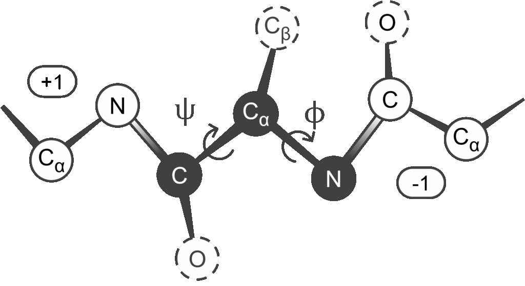
• For proteins, each amino acid can be represented by the coordinates of just its alpha carbon (C_α). For nucleic acids, one might take each nucleotide and represent it by the position of its phosphate group or by the center of its base or sugar ring.
• Another example of controlled granularity comes from how AlphaFold [49] represents protein using backbone rigid groups (or frames). Essentially, for each amino acid, a small set of main-chain atoms, typically the N, C_α, C (and maybe O) are treated as a unit. The relative geometry of these atoms is almost fixed (covalent bond lengths and angles don’t vary significantly), so that unit can be considered as a rigid block. Instead of tracking each atom separately, the model tracks the position and orientation of that entire block in space, reducing the risks associated with excessive degrees of freedom [28] (i.e., errors from the internal movement of atoms within a residue).

• If we have a large set of protein structures (or a long molecular dynamics trajectory), it can be useful to cluster those conformations into a few representative states. This is often done when building Markov state models: by clustering continuous states into a finite set of discrete “metastable” states, we can simplify a complex energy landscape into a network of a few states connected by transition probabilities.

Many coarse-grained molecular dynamics force fields, such as MARTINI [50] and UNRES [51], have been developed to represent structural details using fewer particles.

• To capture for side-chain effects without modelling all internal atoms or adding excessive degrees of freedom, a common approach is to represent each side-chain with a single point, typically its center of mass [52]. Such side-chain centroid models are often used in conjunction with backbone models.
• The 3Di Alphabet introduced by Foldseek [53] defines a 3D interaction “alphabet” of 20 states that describe protein tertiary interactions. Thus, a protein’s 3D structure can be converted into a sequence of 20 symbols; and two structures can be aligned by aligning their 3Di sequences.
• We may spatially crop or focus on just part of a biomolecule. For instance, if we’re studying how a small drug molecule binds to a protein (say, in a dataset like PDBBind [54], which is full of protein-ligand complexes), we may only feed the pockets and drugs into our model.
• Combining different granularities or modalities of data.

Point Cloud

We could model a biomacromolecule as a massive 3D point cloud of every atom (or residue). As noted earlier, the same limitations apply.

Distance Matrix

A distance matrix records all pairwise distances between certain key atoms (for proteins, commonly the C_α of each amino acid), and is inherently invariant to rotation and translation due to its symmetric nature. A contact map simplifies this further by indicating only which pairs of residues are “close enough” to be in contact. However, both representations lose directional information; so not all structural details can be recovered from them alone.

Graph

Similarly, just like we can use graphs for small molecules, we can use graphs for macromolecular structures [55,56]. Instead of atoms, each node might represent a larger unit (see Granularity and Dimensionality Control). To improve interpretability, additional knowledge like residue descriptors and known interaction networks within a protein, may also be incorporated in nodes and edges. Note that the graph representation for biomacromolecules inherits many of the advantages we discussed for small molecules.

For macromolecules, edges are often pruned to keep the graph sparse and manageable in size: essentially a form of local magnification that focuses on local substructures, while far-apart relationships are treated as background context.

General dimensionality reduction methods such as PCA, t-SNE and UMAP are also widely used to analyze the high-dimensional structural data of macromolecules. While they don’t give us representations for computation in the same sense as the others we’ve discussed, they help project complex data into lower dimensions (e.g., for visualization or insights).

Latent Space

When we train a model (especially generative models), it often learns to encode data into a compressed internal representation. This internal representation lives in some space of lower dimension, known as the latent space. Think of London’s complex urban layout, dense and intricate, while the latent space is like a “map” that captures its essence in a simplified form.

Latent spaces are usually not directly interpretable, but we can explore them by seeing how changes in latent variables map to changes in the output. In molecular generation, if a model maps molecules into a latent space, we can take two molecules (say, as two points in that space) and generate a path between them. Ochiai et. al. [57] did this by taking two known molecules as endpoints, interpolating between their latent representations, and decoding the intermediate points. The result was a set of new molecules that blended features of both originals: hybrids that might have mixed properties of the two.